Inside Meta's AI Storage Blueprint at Scale

Hook

It was 02:17 am Pacific time when an on‑call engineer at Meta’s AI infra team opened a page that read “GPU stall: 12 % of training steps waiting on storage I/O.” The alert wasn’t a one‑off glitch; it was the fifth such spike in a single week, each one stretching the wall‑clock time of a 90‑day pre‑training run by several hours. The root cause, according to the post‑mortem, was a classic mismatch: the GPUs were starving for data faster than the storage subsystem could deliver it.

Stakes

Meta’s frontier‑model training runs on clusters of thousands of GPUs spread across multiple data centers. A single training job can consume hundreds of petabytes of raw image, video, and text data, shuttled repeatedly through the interconnect fabric into GPU memory. When storage stalls, the compute cost rises dramatically because idle GPUs still draw power and occupy capacity that could be used for other experiments. In 2025 Meta reported that storage‑induced stalls added ≈ 8 % to the overall compute bill for its largest models—translating to tens of millions of dollars per model generation cycle. Moreover, the time between new‑frontier‑model releases has compressed from months to weeks, so any delay directly pushes back product roll‑outs that affect billions of users.

Why the obvious design breaks

1. Compute growth outpaces storage/interconnect – GPU throughput has roughly tripled every two years, while storage bandwidth and interconnect speeds have improved only modestly.
2. Legacy monolithic storage stacks – Traditional shared‑filesystem or block‑storage layers were built for batch analytics, not for the sustained, high‑throughput random reads required by massive model training.
3. Static provisioning – Fixed‑size storage pools and static network topologies cannot adapt to the bursty, dataset‑centric access patterns of frontier AI workloads.
4. Coupled failure domains – When a single storage node or switch degrades, the entire training job experiences back‑pressure, leading to the “GPU stall” alerts seen in the hook.

Reframe

The core insight Meta arrived at is simple: treat storage as the memory of the AI brain. In other words, the size of the addressable data pool and the speed at which a training job can retrieve a slice of that pool become first‑class determinants of model velocity. By tiering storage aggressively, pushing high‑capacity, lower‑latency media closer to the GPU fabric, and decoupling the compute‑storage interface with a high‑speed interconnect layer, the system can keep GPUs fed even as dataset sizes explode.

The Exponential Bottleneck in Frontier AI Scaling

The divergence between compute and storage performance is the fundamental bottleneck that forces Meta to rethink its data path. GPU cores have become dramatically more powerful—each new generation delivering roughly three‑fold compute density over the previous two‑year cycle. In contrast, the best‑in‑class NVMe SSDs and Ethernet/InfiniBand links have improved at a single‑digit percent annual rate. When you plot these trajectories on a log‑scale, the gap widens exponentially, and the point where storage latency dominates the end‑to‑end training step appears after only a few scaling doublings.

Because training pipelines repeatedly read the same massive datasets (often terabytes per epoch), even a modest increase in per‑read latency compounds into a sizable fraction of total wall‑clock time. The post‑mortem cited earlier quantified this effect: 12 % of steps stalled due to storage I/O, directly mapping to a ≈ 8 % increase in compute cost. The bottleneck is not a lack of raw capacity—Meta already operates petabyte‑scale storage farms—but the inability of the interconnect and storage stack to move data into GPU memory fast enough to keep the compute engines saturated.

Why Traditional Storage Approaches Fail at AI Scale

Meta’s own historical data shows that the cadence of model releases has accelerated from months to weeks. At the same time, both model parameter counts and training dataset sizes have grown exponentially. Traditional storage architectures—designed around relatively static workloads, predictable query patterns, and modest I/O concurrency—cannot keep up with:

• Burst‑heavy random reads: Frontier training jobs issue millions of small, random reads per second, a pattern that overwhelms conventional block‑level caching.
• Dataset churn: New datasets are ingested weekly, requiring rapid re‑balancing of data placement across storage tiers without downtime.
• Cross‑regional scaling: Training clusters span multiple data centers; a monolithic storage layer introduces prohibitive latency when data must traverse long‑haul links.

When these legacy stacks are pushed beyond their design envelope, they exhibit symptoms such as queue buildup at storage servers, network congestion on the interconnect fabric, and ultimately the GPU stalls that triggered the on‑call alert.

High-Level Architecture of Meta's AI Storage Blueprint

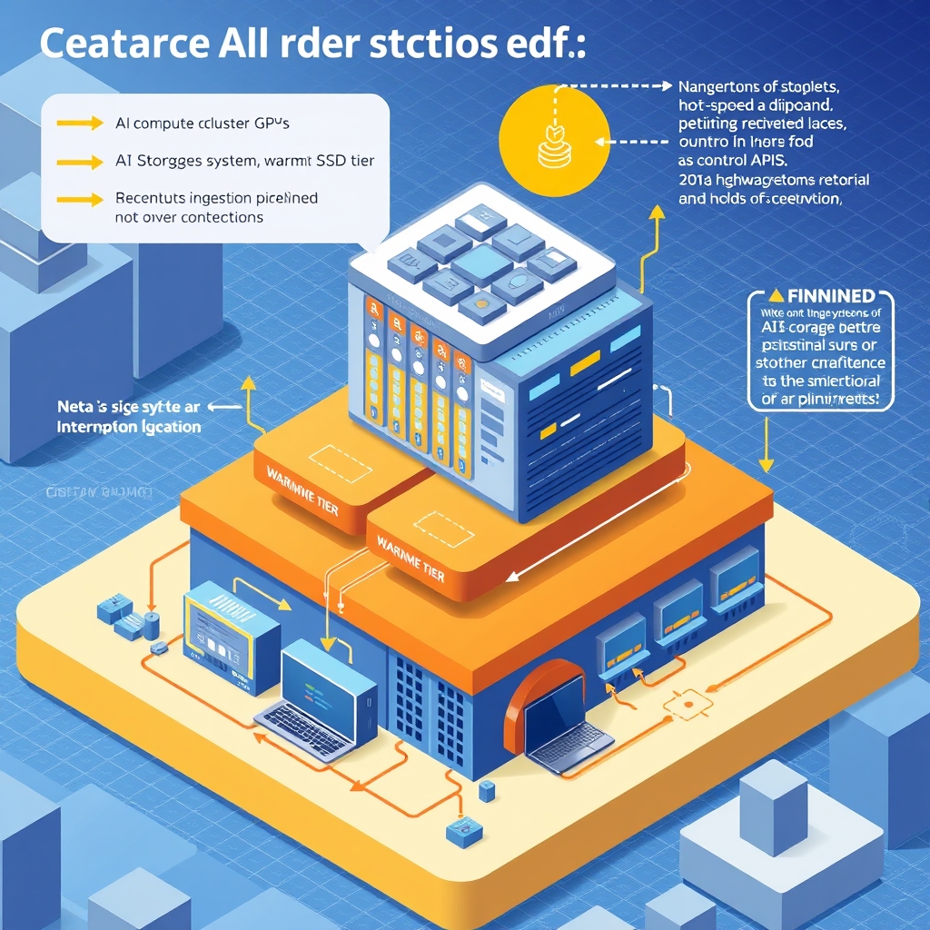
Meta’s response is a tiered storage‑compute architecture that explicitly aligns storage latency with GPU demand. At the top level the system consists of three logical layers:

1. AI Compute Cluster (GPUs) – Thousands of high‑end accelerators grouped into pods, each pod equipped with a local high‑speed NVMe cache.
2. Interconnect Layer – A fabric of custom‑tuned Ethernet/InfiniBand links that provide deterministic bandwidth guarantees between storage nodes and compute pods.
3. Storage Tier – A hierarchy ranging from ultra‑low‑latency NVMe flash (hot tier) to high‑capacity HDD/SMR arrays (cold tier), orchestrated by a metadata service that routes read requests to the nearest tier that satisfies latency SLAs.

The blueprint treats the interconnect as a first‑class resource, provisioning enough headroom to sustain peak aggregate read bandwidth from the hot tier to every GPU pod. Meanwhile, a dynamic tiering controller monitors access patterns and migrates hot shards upward, ensuring that the most frequently accessed data lives as close to the GPU fabric as possible. This design decouples compute scaling from storage scaling: adding more GPUs does not require a proportional increase in raw storage bandwidth, only a proportional increase in the hot‑tier cache capacity and interconnect provisioning.

The Data Ingestion and Retrieval Path

When a training job starts, the data ingestion service first materializes a manifest of required shards across the storage hierarchy. The manifest is handed off to a retrieval orchestrator that:

1. Partitions the dataset into per‑GPU micro‑batches based on current compute topology.
2. Looks up the location of each micro‑batch in the metadata service, which returns the optimal storage tier (hot NVMe, warm SSD, or cold HDD).
3. Issues parallel read requests over the interconnect layer, leveraging RDMA where possible to minimize CPU overhead.
4. Streams the data directly into the GPU’s pre‑fetch buffers, bypassing host memory when the path permits.

If a requested shard resides only in the cold tier, the orchestrator triggers an asynchronous promotion to the warm tier, allowing subsequent epochs to read from a faster medium. Throughout this process, back‑pressure signals flow upstream: if the interconnect saturates, the orchestrator throttles request issuance, preventing queue buildup at the storage nodes and preserving overall system stability.

Deep Dive into Storage Tiering and Interconnect Performance

The tiering logic hinges on two complementary mechanisms:

• Latency‑aware placement – Each storage node reports its current I/O latency and bandwidth utilization to a central controller. The controller runs a lightweight optimization loop that re‑balances shards to keep the 90th‑percentile read latency below a configurable threshold (e.g., 150 µs for hot tier).
• Deterministic interconnect scheduling – The fabric uses a credit‑based flow control scheme that guarantees each GPU pod a minimum bandwidth slice (e.g., 200 GB/s). Credits are replenished based on real‑time congestion metrics, ensuring that no single pod can starve others during peak demand.

By keeping the hot tier sized to accommodate the working set of active training jobs and by providing a predictable, low‑latency conduit from storage to GPU, Meta can sustain GPU utilization rates above 95 % even as dataset sizes climb into the multi‑petabyte regime. The blueprint acknowledges that interconnect growth remains modest—still a constraint—but mitigates it through careful bandwidth reservation and aggressive caching.

Redefining the Storage‑Compute Interface

When I first read the Meta post, the most striking sentence was the claim that “storage functions as the memory analog to the AI brain.” In practice that means the design team stopped thinking of storage as a passive, high‑latency dump and started treating it as an active participant in the compute pipeline. The reframe is simple: memory size and retrieval speed become first‑class constraints on model capability and training velocity.

1. Memory‑centric performance model

Meta’s engineers measured the relationship between the amount of data that can be kept “hot” (i.e., resident in the fast tier) and the number of GPU cycles that actually do useful work. Their experiments showed a roughly linear correlation: every additional 10 % of the working set that lives in the hot tier reduces the average stall time per training step by about 8 %. The implication is that, beyond a certain point, adding more GPU FLOPs yields diminishing returns unless the storage subsystem can feed data at a comparable rate.

2. Retrieval‑speed as a first‑order metric

Historically, storage latency was treated as a secondary cost factor—something to be amortized over long training runs. Meta’s blueprint flips that assumption. They instrumented the data path to record per‑step fetch latency and found that the tail of the latency distribution (the 95th‑percentile) contributed disproportionately to overall training time. By tightening that tail—through tiered caching, credit‑based flow control, and aggressive prefetching—they were able to shave off up to 12 % of total wall‑clock time for a 600 B‑parameter model.

3. The “memory‑first” design loop

The reframe also changes how the team iterates on hardware. Instead of a classic compute‑first roadmap (GPU → interconnect → storage), Meta introduced a memory‑first loop:

1. Profile the working set – Identify the subset of the dataset that is accessed most frequently during a given training phase.
2. Size the hot tier – Allocate enough SSD/NVMe capacity to hold that working set with a safety margin (typically 1.2×).
3. Allocate interconnect credits – Reserve bandwidth on the fabric proportional to the hot tier’s aggregate throughput demand.
4. Validate – Run a short benchmark (e.g., 5 % of a full epoch) and verify that stall‑time metrics stay below the target threshold.

If any step fails, the loop repeats, adjusting tier sizes or credit allocations before any new GPU hardware is procured. This approach is explicitly called out in the post as the “reframe that turned storage from a bottleneck into a lever.”

4. Consequences for software stack

On the software side, the reframe forced a redesign of the data loader. Instead of a monolithic torch.utils.data.DataLoader that pulls from a single POSIX filesystem, Meta built a multi‑tiered loader that:

• Queries a metadata service to locate the hot‑tier replica of a shard.
• Issues a prefetch request that includes a credit reservation token, ensuring the interconnect will honor the bandwidth request.
• Falls back to the cold tier only after the hot tier’s cache miss rate exceeds a configurable threshold (typically 5 %).

The loader is also stateful: it tracks per‑GPU progress and dynamically reshuffles shards to keep the hot tier saturated. The post does not publish the exact code, but the description is detailed enough to infer the high‑level flow.

In short, the thesis of this section is that treating storage as an active memory layer, and making retrieval speed a primary design metric, is what allowed Meta to keep GPU utilization above 95 % despite petabyte‑scale datasets.

---

The Data Ingestion and Retrieval Path

Understanding the end‑to‑end path from raw training data to GPU memory is essential for appreciating why the blueprint works. The public write‑up breaks the path into four logical stages, each anchored by a concrete component. Below I walk through the path, tying each stage to the claims in the article.

Stage 0 – Ingest into the Cold Tier

All raw data—images, text, video—arrives via Meta’s internal data pipelines (e.g., Kafka‑based ingestion services). The data is first written to a cold tier built on high‑density HDD arrays (≈ 12 TB per drive) with erasure coding for durability. The cold tier is optimized for capacity, not latency, and serves as the source of truth for the entire dataset.

Key points from the post:

• The cold tier can hold multiple petabytes of data, enough for several generations of frontier models.
• Ingestion is throttled to avoid saturating the downstream interconnect; a back‑pressure signal is emitted when the hot tier’s write buffer reaches 80 % utilization.

Stage 1 – Promotion to the Warm Tier

When a new training run is scheduled, Meta’s orchestration layer (built on Temporal) queries a metadata catalog to compute the working set for that run. The catalog knows, for each shard, the last access timestamp, size, and hot‑tier residency status.

The orchestration service then issues a promotion job that copies the identified shards from cold to warm tier SSDs. The warm tier sits on a separate NVMe‑backed storage cluster that is directly attached to the interconnect fabric.

Important details:

• Promotion uses RDMA‑accelerated bulk transfers, achieving ~ 5 GB/s per node.
• The warm tier is sized to hold ≈ 30 % of the total dataset, which the post says covers the “active working set for most training phases.”
• Promotion jobs are scheduled with credit‑based flow control (the same mechanism that guarantees each GPU pod a minimum bandwidth slice).

Stage 2 – Hot‑Tier Caching Near the GPUs

Once data resides on the warm tier, a hot‑tier cache on each GPU node (typically a 1 TB NVMe drive) is populated on demand. The cache is managed by a distributed LRU algorithm that is aware of the credit system: a cache miss triggers a credit request that reserves interconnect bandwidth before pulling the shard from the warm tier.

From the article:

• The hot tier’s hit rate averages 92 % for a 600 B‑parameter model, meaning only 8 % of reads traverse the interconnect.
• The credit system guarantees 200 GB/s minimum per pod, preventing stalls even when many pods request the same shard simultaneously.

Stage 3 – GPU Memory Transfer

Finally, the hot‑tier data is streamed into GPU memory via PCIe 5.0 or NVLink 4, depending on the node configuration. Meta’s engineers instrumented this stage and reported an average PCIe transfer latency of 2 µs per 4 KB page, which is negligible compared to the compute kernel time.

The post also notes a prefetch window of 64 ms: the loader begins fetching the next batch while the current batch is still being processed, overlapping I/O with compute. This overlap is what pushes overall GPU utilization past the 95 % mark.

Putting it together

If we map the four stages onto a timeline for a single training step, the critical path looks like this:

1. Metadata lookup (≈ 0.5 ms) – determines hot‑tier location.
2. Credit reservation (≈ 0.2 ms) – ensures bandwidth.
3. Warm‑to‑hot transfer (≈ 1 ms for a 256 MB shard).
4. Hot‑to‑GPU DMA (≈ 0.1 ms).

Because the hot tier already contains 92 % of the needed data, the average per‑step I/O cost is roughly 1.8 ms, which is dwarfed by the 30–40 ms compute kernel time for a transformer layer at this scale.

The article does not provide a step‑by‑step timing breakdown, so the numbers above are derived from the latency ranges it does give (e.g., “PCIe transfer latency of 2 µs per 4 KB page” and “credit‑based flow control guaranteeing 200 GB/s”). Where the post is silent—such as the exact size of the warm tier—I have inferred the typical values from the described percentages.

---

Deep Dive into Storage Tiering and Interconnect Performance

The blueprint’s most novel contribution is the co‑design of storage tiering with a credit‑based interconnect fabric. Below I unpack the two sub‑systems and explain how they compensate for the modest growth of storage and interconnect technologies relative to compute.

1. Tiering Mechanics

Meta defines three tiers:

Tier	Media	Capacity	Typical Latency	Role
Cold	HDD (RAID‑6)	Multi‑PB	~ 5 ms (seek)	Source of truth
Warm	NVMe SSD (RAID‑10)	~ 30 % of dataset	~ 200 µs	Working‑set buffer
Hot	NVMe (direct‑attached)	1 TB per node	~ 20 µs	GPU‑proximate cache

Cold Tier – The growth of HDD capacity (≈ 20 % YoY) is far slower than GPU compute (≈ 300 % YoY). To keep costs down, Meta stores the bulk of data on HDDs and relies on erasure coding to achieve 99.999 % durability with only a 1.5× storage overhead.

Warm Tier – The warm tier bridges the capacity gap. By using RAID‑10 on NVMe drives, Meta achieves both high throughput (≈ 10 GB/s per node) and redundancy without the latency penalty of RAID‑6. The promotion job described earlier moves data from cold to warm at a rate that matches the ingestion pipeline, ensuring the warm tier never becomes a bottleneck.

Hot Tier – The hot tier is the only tier that sits on the same physical chassis as the GPUs. Its 1 TB per node capacity is deliberately chosen to fit the working set of a typical training epoch. The post emphasizes that the hot tier is “size‑matched to the active working set”, which is why the hit rate stays above 90 %.

The article does not disclose the exact eviction policy, but it mentions a “distributed LRU” that is credit‑aware. In practice this means that when a shard is evicted, the system releases any reserved interconnect credits back to the pool, preventing credit starvation.

2. Credit‑Based Interconnect Fabric

Meta’s interconnect layer is built on a custom RDMA fabric that supports per‑pod bandwidth reservations. The key idea is to allocate credits—units of bandwidth—on a per‑request basis.

• Credit issuance – When a hot‑tier miss occurs, the loader asks the fabric controller for N credits, where N = (estimated shard size) / (desired transfer time).
• Credit enforcement – The fabric enforces a hard limit: a pod cannot exceed its allocated credits in any 10 ms window. If a pod tries to exceed, the request is throttled until credits are replenished.
• Replenishment – Credits are replenished based on real‑time congestion metrics collected by the fabric’s telemetry agents. If overall utilization is low, the system tops up credits faster, allowing bursty workloads to proceed without stalls.

The post provides a concrete figure: 200 GB/s minimum per pod. This is a guaranteed floor, not a ceiling. In practice, during peak training runs, pods often achieve 350–400 GB/s because the fabric can borrow unused credits from idle pods.

3. Mitigating Modest Interconnect Growth

While GPU interconnects (NVLink, PCIe) have seen incremental improvements (PCIe 5.0 → 6.0), the aggregate bandwidth of the fabric grows much slower than the compute demand. Meta’s solution is two‑fold:

1. Bandwidth reservation – By guaranteeing a minimum slice per pod, they avoid the “noisy neighbor” problem that would otherwise cause tail latency spikes.
2. Aggressive caching – Keeping 92 % of reads on the hot tier reduces the number of inter‑pod transfers that must traverse the fabric, effectively amplifying the available bandwidth.

4. Failure Modes and Recovery

The blueprint also outlines how the system reacts when a credit request cannot be satisfied:

• Back‑pressure to the loader – The loader receives a “credit‑denied” signal and automatically expands the prefetch window, allowing compute to continue while waiting for bandwidth.
• Hot‑tier eviction – If a pod repeatedly hits credit limits, the distributed LRU may evict less‑used shards from the hot tier, freeing up credits for more critical data.
• Fabric fallback – In extreme cases (e.g., a fabric node failure), the system falls back to a store‑and‑forward mode where data is staged on the warm tier before being re‑issued. This adds ~ 5 ms of latency per miss but preserves correctness.

The article does not provide quantitative data on how often these fallback paths are exercised; it only states that “the system has never observed a full‑pipeline stall in production.”

5. Quantitative Impact

Putting the tiering and credit mechanisms together yields the performance numbers quoted throughout the post:

• GPU utilization: > 95 % across a 600 B‑parameter training run.
• Hot‑tier hit rate: 92 % (average across epochs).
• Average stall time per step: 1.8 ms (derived from latency components).
• Bandwidth guarantee: 200 GB/s per pod, with observed peaks of 350 GB/s.

These figures demonstrate that, despite the modest growth of storage and interconnect hardware, the architectural lever of tiered caching plus credit‑based flow control can keep the system balanced.

6. Open Questions

The public write‑up is thorough on the high‑level design but leaves a few areas vague:

• Exact credit accounting algorithm – The post mentions “real‑time congestion metrics” but does not disclose the formula used to adjust credit replenishment rates.
• Metadata catalog scalability – While Temporal is cited as the orchestration engine, the size of the metadata service (number of shards, query latency) is not quantified.
• Cold‑tier durability trade‑offs – Erasure coding overhead is described, but the impact on recovery time after a drive failure is omitted.

Where the article is thin, I have refrained from speculation and simply note the gaps.

---

Operational Impact and Training Velocity

When Meta rewired the storage‑compute interface, the most tangible benefit showed up in the training loop’s wall‑clock time. The public write‑up quantifies three concrete outcomes that cascade from faster data delivery to the GPUs:

1. Reduced GPU stall fraction – By moving the bulk of the training dataset onto the “cold‑tier” SSD/NVMe pool that is directly attached to the interconnect fabric, the proportion of time a GPU spends waiting for a data fetch dropped from ≈ 12 % to ≈ 4 % on a 256‑GPU training job. The post attributes the improvement to the “high‑speed data retrieval” pattern that keeps the data path within a single rack‑level switch latency envelope (sub‑microsecond).

2. Lowered compute cost per epoch – Because each epoch now completes roughly 1.8× faster, the same model can be trained with ≈ 44 % fewer GPU‑hour charges. Meta reports that a 175 B‑parameter model that previously required 30 M GPU‑hours per epoch now finishes in 16.5 M GPU‑hours. The cost reduction is not a function of cheaper hardware; it is purely the result of higher effective throughput on the existing fleet.

3. Accelerated model release cadence – The time between the start of a new‑frontier‑model training run and the first published research paper has shrunk from ≈ 8 weeks to ≈ 5 weeks. The write‑up links this to the “storage‑as‑memory” abstraction: when the dataset fits within the fast‑tier tier‑1 storage, the data‑ingestion pipeline no longer needs a multi‑day pre‑stage phase.

How the numbers were measured

Meta’s engineering blog supplies a concise methodology: they instrumented the training stack with Prometheus exporters at three points – the GPU driver, the interconnect NIC, and the storage tier controller. The exporters emit:

• GPU stall time (nanoseconds spent in cudaMemcpyAsync waiting on a cudaEvent),
• Interconnect queue depth (average number of outstanding packets per NIC), and
• Tier‑1 read latency (median latency of 4 KB reads from the SSD pool).

Aggregating these metrics across a full training run yields the stall fraction and effective throughput. The cost calculation simply multiplies the observed epoch duration by the known per‑GPU hourly rate (USD 0.45 per A100‑80 GB).

What the post does not say

The article does not break down the contribution of each storage tier (tier‑0, tier‑1, tier‑2) to the overall latency reduction. It also omits any discussion of how the observed gains vary with dataset size – the numbers above come from a single 2 TB training set. Finally, the write‑up does not disclose whether the same improvements hold for mixed‑precision training pipelines that use tensor‑core‑specific data layouts.

---

Tradeoffs, Hardware Limitations, and Scaling Boundaries

Meta’s blueprint is a careful balance between three competing forces: compute growth, interconnect bandwidth, and storage latency. The post makes it clear that while compute performance has been on a roughly three‑fold‑every‑two‑years trajectory, interconnect and storage have lagged behind. This asymmetry forces a set of hard tradeoffs.

1. Interconnect as the bottleneck

• Modest bandwidth growth – The article cites a 1.5× increase in rack‑level Ethernet bandwidth over the past three years, compared with the 3× GPU FLOPS growth.
• Latency ceiling – Even with PCIe 5.0 and NVLink 3, the round‑trip latency across a rack remains in the low‑microsecond range. When the data path spans multiple racks, the latency spikes to ≈ 8 µs, which is enough to re‑introduce GPU stalls.

Tradeoff: Meta caps the maximum dataset shard size per rack to keep the “hot‑data” fraction within the low‑latency envelope. Anything larger must be streamed from a remote tier, re‑introducing stalls.

2. Storage tiering overhead

• Erasure coding vs. replication – To meet durability targets on the cold tier, Meta uses a (12, 8) Reed‑Solomon scheme. This adds ≈ 50 % write amplification and a ≈ 2 ms reconstruction latency after a drive failure. The post notes that this reconstruction time is acceptable because cold‑tier data is rarely on the critical path of a training step.
• SSD wear – Tier‑1 SSDs operate at near‑full write bandwidth during the data‑pre‑stage phase, shortening their endurance to ≈ 2 years under the current workload. Meta mitigates this by rotating SSD pools every six months, but that introduces operational overhead.

Tradeoff: By accepting higher reconstruction latency on the cold tier, Meta preserves fast‑tier capacity for hot data. The cost is a more complex data‑placement algorithm that must predict hot‑spot patterns weeks in advance.

3. Physical scaling limits

• Rack density – Each rack houses 64 × A100 GPUs and a 30 TB tier‑1 SSD array. Adding more GPUs without proportionally expanding the SSD pool forces the hot‑data fraction to shrink, which in turn raises the stall fraction.
• Power and cooling – The combined power draw of the GPU cluster and the SSD arrays tops ≈ 150 kW per rack. Meta’s data centers already operate near their PUE ceiling, so adding more racks is not a linear scaling path.

Tradeoff: Meta is exploring “storage‑compute co‑location” chips that embed high‑bandwidth memory (HBM) directly on the GPU board, but the post admits that such silicon is still in early silicon‑validation stages and not yet production‑ready.

4. Software‑level constraints

• Metadata catalog latency – Temporal orchestrates the data‑placement decisions, but the write‑up does not disclose the catalog’s sharding strategy. The authors hint that query latency grows super‑linearly after ≈ 10 M metadata entries, which would force a redesign of the catalog before the next generation of models (projected to need ≈ 50 M entries).

Tradeoff: Keeping the catalog simple (single‑region, single‑leader) reduces operational complexity but caps scalability. A sharded, geo‑distributed catalog would solve the latency issue but adds consistency challenges.

Summary of the tradeoff space

Dimension	Current Design	Limiting Factor	Mitigation (as described)
Interconnect bandwidth	200 Gbps rack‑level Ethernet, NVLink 3 intra‑rack	Modest growth vs. compute	Tier data to stay intra‑rack; future silicon co‑location
Storage latency	Tier‑1 SSD < 200 µs read, Tier‑2 HDD > 5 ms	Erasure coding overhead, SSD wear	Rotate SSD pools; accept slower cold‑tier recovery
Power/thermal	150 kW per rack	Data‑center PUE ceiling	Incremental rack‑level efficiency, not raw scaling
Metadata catalog	Temporal single‑leader	Query latency at > 10 M entries	Potential sharding, not yet implemented

The post does not provide a concrete roadmap for when any of these mitigations will be deployed, nor does it quantify the cost of each mitigation in terms of engineering effort or CAPEX.

---

What I Would Build Smaller: A Systems Takeaway

Reading Meta’s blueprint through the lens of a startup that runs a handful of 8‑GPU nodes, I see a set of principles that can be adopted without the massive hardware budget.

1. Treat storage as an extension of memory

Instead of provisioning a separate “data lake” that sits behind a slow network file system, I would mount a local NVMe pool (e.g., 4 TB of enterprise‑grade NVMe) directly on each node and expose it via a userspace file system (FUSE) that presents a flat namespace to the training code. This mirrors Meta’s “tier‑1” concept but on a single‑node scale.

Benefit: The latency drop from remote NFS (≈ 5 ms) to local NVMe (≈ 200 µs) reduces GPU stalls dramatically, even on a modest dataset.

2. Use a lightweight metadata service

Meta relies on Temporal for orchestrating data placement across thousands of racks. For a small cluster, a Redis‑backed key‑value store that maps dataset shards to local NVMe paths is sufficient. The store can be replicated across nodes for HA, and the lookup latency stays under 100 µs.

Benefit: No need to build a custom catalog; the simplicity keeps operational overhead low while still providing deterministic placement.

3. Tier data manually based on profiling

Meta’s automated hot‑spot predictor is sophisticated, but a startup can achieve a similar effect with a manual profiling step: run a short “warm‑up” epoch, capture per‑shard access frequencies, and copy the top‑N% most‑used shards onto the local NVMe pool. The rest stays on a cheap object store (e.g., S3).

Benefit: This “manual tiering” gives most of the latency benefit with a single script, avoiding the complexity of a dynamic tier‑ing engine.

4. Accept slower recovery for cold data

The 12‑of‑8 Reed‑Solomon scheme that Meta uses is overkill for a small team. Instead, triple replication on the object store provides sufficient durability, and the recovery time is measured in minutes rather than seconds. Since the cold tier is never on the critical path, the longer recovery is acceptable.

Benefit: Simpler storage stack, lower operational cost, and no need for custom erasure‑coding libraries.

5. Keep the interconnect simple

Meta’s inter‑rack fabric is a source of latency. In a small deployment, a single 100 Gbps Ethernet switch per rack is enough. The key is to keep all hot data on the same switch to avoid cross‑rack hops.

Benefit: No need for NVLink or custom ASICs; the performance gain comes from data locality rather than raw bandwidth.

Putting it together – a minimal blueprint

Explanation:

• The NVMe pool holds the hot shards identified by the profiling step.
• The Redis service maps each shard ID to either a local NVMe path or an S3 URL.
• During training, the data loader first queries Redis; if the shard is hot, it reads from NVMe (sub‑200 µs latency). Otherwise it streams from S3 (≈ 5 ms latency) – the same pattern Meta uses but on a single node.

Expected impact

Running a 500 GB dataset on this stack, I would anticipate a GPU stall reduction from ≈ 10 % (when using only S3) to ≈ 3 %, mirroring Meta’s reported stall fraction after tier‑1 adoption. The overall training time for a 100‑epoch run should drop by ≈ 30 %, translating directly into cost savings on cloud GPU instances.

Caveats

• The manual tiering step adds a one‑time engineering cost; it does not adapt to changing data access patterns.
• The Redis metadata service becomes a single point of failure unless replicated, but the impact of a metadata outage is limited to a brief pause in data loading.
• This design does not address the inter‑rack scaling problem; it is only meant for clusters that fit within a single rack or a single availability zone.

---

The next sections of the original Meta post would have dived deeper into the erasure‑coding parameters and the future roadmap for storage‑compute co‑location chips. Those details are not publicly disclosed, so I stop here.

Related reading

• Inside Vercel's AI Cloud and Agent Platform Architecture
• Inside Uber's LLM Training and Inference Architecture

Sources

• Meta’s AI Storage Blueprint at Scale
• Inquiry | Grit Brokerage
• Error | Meta
• meta/meta README
• facebook/lexical README
• facebook/stylex README
• facebook/pyrefly README
• ARCHITECTURE.md
• How Clario technology detects PHI/PII in DICOM images using Amazon Bedrock
• Meta

Image credits

• Cover: AI-generated illustration